Linear Discriminant Function and How to compute it?

Linear Discriminant functions

Linear Discriminant functions are the basis for the majority of Pattern Recognition techniques. It is a function that maps input features onto a classification space.
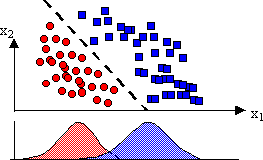
A dividing boundary that separates two clusters (group) are shown below-

The mathematical definition of such a decision boundary is a Discriminant function. A linear Discriminant (LD) is a linear combination of the components of x ={x1,x2….xd } given by a weight vector, w ={w1,w2….wd}, and a bias parameter, w0, also known as the threshold weight.

Then LD can be written as:
g(x)= wtx+w0 or as: g(x) = (w, x) + w0
In the simplest classification scenario we have two classes, the decision rule of a LD is:
– If g(x) > 0 then x is classified w1
– If g(x) < 0 then x is classified w2
g(x) = 0 defines the decision surface that separates the two classes. When g(x) is linear the decision surface, i.e. g(x), is a hyperplane.

How to Compute g(x)?
There are many different ways to compute the w, and w0, needed for the definition of g(x). Just some of them:
 Bayes Theorem
 Fisher’s linear discriminants
 Perceptrons
 Logistic Regression
 Support Vector Machines

 Minimum squared error (MSE) solution
 Least-mean squares (LMS) rule
 Ho-Kashyap procedure.

Linear Discriminant Function using Bayes Theorem

C= (g1(x), g2(x)…..gn(x))
wi: i=argmax(gi(x))
where, gi(x)= p(wi|x)
Discriminants DO NOT have to relate to probabilities.

For two-class problem:
Classes: w1, w2.
g1(x)= p(w1|x) ; g2(x)= p(w2|x) ; g(x)= g1(x)- g2(x)
Then (assuming that classes are encoded as +1 and -1): wi=sign(g(x)) i.e., Classify x in w1 if g(x)>0 or in w2, otherwise.